The package

Perform fancy statistics by yourself. Correct and fast.

Installation

library(devtools) # Tools to Make Developing R Packages Easier 
devtools::install_github("Watjoa/CaviR")

Correlations

Using the coRtable function to have a clear, informative correlation table with descriptions

coRtable(data[,c("Extra","Agree","Con","Neur","Open")])

	M	SD	1.	2.	3.	4.	5.
1. Extra	3.58	0.52
2. Agree	3.66	0.53	.22*
3. Con	3.43	0.54	.06	.42***
4. Neur	2.76	0.8	.06	-.19	-.28**
5. Open	3.41	0.58	.44***	.22*	.27**	.04
Note. *** p <.001, ** p <. 01, * p < .05

or use the multicoR function to have a correlation table for within-group and between-group level. Descriptives are based on the between-group level.

multicoR(datamultilevel[, c(
  "ID","Integration","Suppression","Dysregulation")])

	M	SD	ICC	1.	2.	3.
1. Integration	3.29	0.66	0.64		-.08***	.23***
2. Suppression	2.32	0.76	0.63	-.25***		.15***
3. Dysregulation	2.26	0.73	0.59	.18***	.35***
Note. *** p <.001, ** p <. 01, * p < .05

Tip

In R, you can select the whole output (CTRL+A or CMD+A) and paste the output in excel to provide further modifications.

(M)ANOVA

Using the manovaR function, a descriptive overview is displayed for a comparison between groups, including univariate, multivariate and tukey post-hoc analyses.

manovaR(data[,c('Group','Autonomy','Vitality','Persistence')],
        stand=TRUE, sign = 0.05, tukey = TRUE)

[1] "Grouping variable has only 2 levels. Tukey not applicable"

variables	Group 1	Group 2	F-value	p-value		eta-squared
Autonomy	3.37 (±0.92)	2.31 (±1.09)	57.48	<.001	***	0.37
Vitality	3.37 (±0.92)	2.31 (±1.09)	41.78	<.001	***	0.29
Persistence	3.37 (±0.92)	2.31 (±1.09)	28.18	<.001	***	0.22
Wilks Lambda = 0.607,F(3,95) = 20.479 , p = <.001

Regression

Using the summaRy function, an overview is presented with information regarding your linear (mixed) model

model <- lm(Persistence~ Condition.d * Indecisiveness.c, data=data) 
summaRy(model)

Predictors	coefficients	β	std. error	t-value	p-value
(Intercept)	1.22	0.00	0.32	3.82	<.001	***
Condition.d	1.10	0.49	0.2	5.56	<.001	***
Indecisiveness.c	1.18	0.64	0.52	2.29	0.02	*
Condition.d:Indecisiveness.c	-0.83	-0.72	0.32	-2.57	0.01	**
ANOVA:
	Sumsq	Meansq	(df)	F stat	partial η2	VIF
Condition.d	28.41	28.41	1	31.11, p = <.001	0.25	1.01
Indecisiveness.c	0.21	0.21	1	0.23, p = 0.63	0.00	10.21
Condition.d:Indecisiveness.c	6.01	6.01	1	6.58, p = 0.01	0.07	10.20
Residuals	83.092	0.913	91
Info: 95 observations, (9) missing obs. deleted
Fit: F(3,91) = 12.64, p = <.001
R2= 0.29, Adj. R2 = 0.27

Significant two-way interaction effects could be displayed using the inteRplot function.

inteRplot(model,
          pred = 'Condition.d',
          mod = 'Indecisiveness.c',
          outcome = 'Persistence',
          xaxis = 'Condition',
          moderator = 'Indecisiveness',
          miny = 1,
          maxy = 5,
          xlabels=c('No choice','Choice'))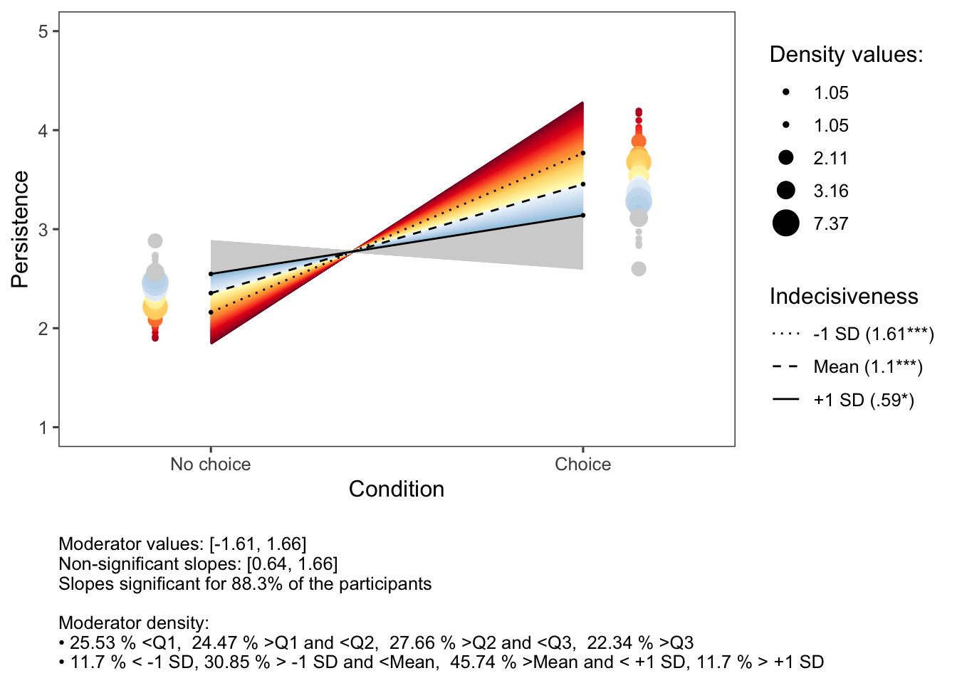 

Clustering

The clusteRsfunction of the CaviR package provides four figures showing a particular type of validation for a number of clusters. Indeed, we want to have all four of them, as we want to make a considered decision on how many clusters are in our dataset. This does not mean that all four types of validations will point towards the same number of clusters (sometimes it does, indicating strong evidence for a particular number). Therefore, you need to consider all types and explain in your reporting why you choose for a particular number of clusters.

What are the validation techniques?

1. Elbow method: the number of clusters with both a minimum of within-cluster variation and a maximum of between-cluster variation
2. the Average Silhouette method: the number of clusters with the highest average silhouette, indicating the best quality of clustering
3. the Gap statistic method: the number of clusters with the highest Gap-statistic [@tibshirani2001]
4. Majority rule: a summary of 30 indices reporting the most optimal number of clusters using the ‘NbClust’ function, including the CH index.

clusteRs(df_clust)