Co-Relate

correlations

netwerk plot

multilevel-correlations

ICC-values

Perform correlation analyses

Author

Joachim Waterschoot

Published

December 3, 2023

Cross-sectional

As no packages were available providing a clean output of a correlation table, including descriptive statistics, I function was constructed in the CaviR package. By using this, a clean table will appear which can be copied wright away in Excel, Word, etc.

Note

First, make a subset of all variables you want to include in the correlation matrix. You can choose which order they have.
Run the coRtable() function

correlation_dataset <- data[, c(
  "Extra","Agree","Con","Neur","Open")]

library(CaviR)
coRtable(correlation_dataset)

	M	SD	1.	2.	3.	4.
1. Extra	3.58	0.52
2. Agree	3.66	0.53	.22*
3. Con	3.43	0.54	.06	.42***
4. Neur	2.76	0.8	.06	-.19	-.28**
5. Open	3.41	0.58	.44***	.22*	.27**	.04
Note. * p <.001, p <. 01, * p < .05

Tip

The output can be opened in Rstudio or in your browser. When copy it (CTRL + A or CMD + A), you can change the layout in your Excel or Word file to whatever you like.

Tip

If you want to change the names of the variables, use colnames(correlation_dataset) <- c(NEW_NAMES) after step 1 where you replace NEW_NAMES by a vector of names you prefer.

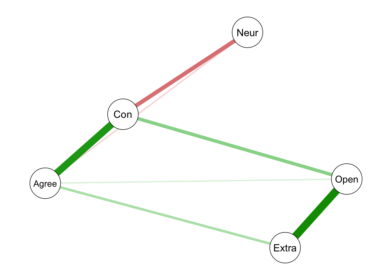
Make a useful netwerk plot based on the variables in the correlation table.

library(qgraph)
corMat <- cor(correlation_dataset, use = "pairwise.complete.obs") # Correlate data
Graph_lasso <- qgraph(corMat, graph = "glasso",
                      layout = "spring", tuning = 0.25,
                      labels = colnames(corMat),
                      sampleSize = nrow(correlation_dataset))

Multilevel correlations

The same CaviR package can be used for multilevel correlations (up until 2 levels).

Note

First, make a subset of all variables you want to include in the correlation matrix. You can choose which order they have, but make sure the grouping variable is the first one.
Run the multicoR() function.

The upper diagonal will present the correlations within levels of the grouping variable. The lower diagonal will do this across groups.

Important

The multicoR function recognizes the first variable as the group variable, so make sure this is the first one in the dataset.

correlation_multileveldataset <- datamultilevel[, c(
  "ID","Integration","Suppression","Dysregulation")]

library(CaviR)
multicoR(correlation_multileveldataset)

	M	SD	ICC	1.	2.	3.
1. Integration	3.29	0.66	0.64		-.08***	.23***
2. Suppression	2.32	0.76	0.63	-.25***		.15***
3. Dysregulation	2.26	0.73	0.59	.18***	.35***
Note. * p <.001, p <. 01, * p < .05

Interpretation:

The table shows high ICC-values, indicating that 64% of the variance in the Integration variable is between groups (i.e., participants in this dataset) and 36% is located within groups, for instance.
Between-group correlations (below diagonal): Group’s overall mean level of Integration (i.e., across time) is related negatively with group’s overall mean on Suppression.
Within-group correlations (upper diagonal): When a person reports a momentary higher level of Integration compared to the overall mean across time, this person also reports a momentary lower level of Suppression compared to the overall mean across time.

Note

The ICC represents the Intra-Class Correlation or the level of between-grouping variable.