Regression modelling

linear modeling

multilevel

interaction plot

simple slopes

johnson-neyman

Perform (multilevel) regression analyses

Author

Joachim Waterschoot

Published

December 4, 2023

Cross-sectional

Time to build our model. Here we have two main effects and one interaction effect of the predictor Condition (i.e., received no choice, received choice) and Indecisiveness (i.e., level of one’s indecisiveness). Condition is a (numeric) dummy code, Indecisiveness is centered. The outcome Pleasure is not centered.

What about categorical predictors: dummy or effect coding?

Before building our model, we need to make sure that all our input is ok. For instance, we want to have dummy or effect codings instead of factor variables. Here, we work with the example of a factor with 3 levels, resulting in 2 dummy codings:

df$dummy1 <- as.factor(df$VAR1)
levels(df$dummy1) <- c(0,1,0)
df$dummy1 <- as.numeric(df$dummy1)

df$dummy2 <- as.factor(df$VAR1)
levels(df$dummy2) <- c(0,0,1)
df$dummy2 <- as.numeric(df$dummy2)

or you want to use effect codings.

To my opinion, this is the most useful one to do as things are centered in our interpretation. When using dummy, you need to interpret the main effect of a particular variable ‘when all other coefficients are kept stable’. In the case of a dummy coding, this means that this refers to the main effect in presence of the reference value of the dummy coding. When doing effect coding, this is not the case and you have a more clear interpretation of the main effect.

df$dummy1 <- ifelse(df$VAR1 == "group2", 1, 0)
df$dummy2 <- ifelse(df$VAR1 == "group3", 1, 0)
df$dummy3 <- ifelse(df$VAR1 == "group4", 1, 0)

What about numeric predictors: center or standardize?

It is to center numeric variables. When centering, you keep the standard deviation. When standardizing, this is forced to 1. This is a choice, but I, personally, like it when the initial variance is kept in terms of interpreting the results.

df$VAR1.c <- as.numeric(scale(df$VAR1,scale=FALSE,center=TRUE))

model <- lm(Persistence~ Condition.d * Indecisiveness.c, data=data)

Important

In this model, we immediatly mentioned the interaction effect because the lm function in R calculates both the main effects and interaction effects by default. This saves time, but beware an interaction effect is not interpretable without main effects in a model.

Check the output of the model using the summaRy function in the CaviR package.

library(CaviR)
summaRy(model)

Predictors	coefficients	β	std. error	t-value	p-value
(Intercept)	1.22	0.00	0.32	3.82	<.001	***
Condition.d	1.10	0.49	0.2	5.56	<.001	***
Indecisiveness.c	1.18	0.64	0.52	2.29	0.02	*
Condition.d:Indecisiveness.c	-0.83	-0.72	0.32	-2.57	0.01	**

ANOVA:
	Sumsq	Meansq	(df)	F stat	partial η2	VIF
Condition.d	28.41	28.41	1	31.11, p = <.001	0.25	1.01
Indecisiveness.c	0.21	0.21	1	0.23, p = 0.63	0.00	10.21
Condition.d:Indecisiveness.c	6.01	6.01	1	6.58, p = 0.01	0.07	10.20
Residuals	83.092	0.913	91

Info: 95 observations, (9) missing obs. deleted
Fit: F(3,91) = 12.64, p = <.001
R2= 0.29, Adj. R2 = 0.27

How to interpret this output?

The output provides several sources of information:

Raw and standardized coefficients
Standard errors and t-values, with p-values
the ANOVA output of the model, providing partial eta-squares and Variance Inflation Factors (to check for multicollinearity)
Number of used observations and how many were excluded from the analyses
Total fit for the model and R-squared values

When selecting the whole output (CTRL + A or CMD + A), one could paste this into Excel or Word.

How to interpret the partial eta-squared?

small when η_p² > .0099
medium when η_p² > .0588
large when η_p² >.1379

(Cohen 2013)

What about model assumptions?

Important is to check to what your model does satisfy all models. A nice way to do this is using the check_model function, however this might take a while (especially in more complex models). You can check all diagnostics separately (which may be faster):

Model assumptions:

Linearity: is my model linear?
- Check?: (1) is the point cloud at random and (2) is the blue line in plot 2 similar to the horizontal line in plot 2?
- Violation?: consider another relationship (e.g. cubric, curvilinear)
Normality: is the distribution of my parameters / residuals normal?
- Check?: do I have a Q-Q plot in plot 3 where all datapoints are as close too the diagonal? Is the distribution as similar as possible to the normal distribution in plot 8?
- Violation?: consider transformations of your parameters or check which variable is necessary to add to the model
Homoscedasticity: is the spread of my data across levels of my predictor the same?
- Check?: (1) is the point cloud at random and (2) is the blue line in plot 2 similar to the horizontal line in plot 2? (3) Is there a pattern in plot 4?
- Violation?: in case of heteroscedasticity, you will have inconsistency in calculation of standard errors and parameter estimation in the model. This results in biased confidence intervals and significance tests.
Independence: are the errors in my model related to each other?
Influential outliers: are there outliers influential to my model?
- Check?: is the blue line in plot 7 curved?
- Violation?: this could be problematic for estimating parameters (e.g. mean) and sum of squared and biased results.

library(performance)
check_normality(model)

Warning: Non-normality of residuals detected (p = 0.031).

check_outliers(model)

OK: No outliers detected.
- Based on the following method and threshold: cook (0.8).
- For variable: (Whole model)

check_heteroscedasticity(model)

OK: Error variance appears to be homoscedastic (p = 0.054).

multicollinearity(model)

# Check for Multicollinearity

Low Correlation

        Term  VIF       VIF 95% CI Increased SE Tolerance Tolerance 95% CI
 Condition.d 1.01 [1.00, 8.59e+09]         1.00      0.99     [0.00, 1.00]

High Correlation

                         Term   VIF       VIF 95% CI Increased SE Tolerance
             Indecisiveness.c 10.21 [7.20,    14.69]         3.20      0.10
 Condition.d:Indecisiveness.c 10.20 [7.20,    14.67]         3.19      0.10
 Tolerance 95% CI
     [0.07, 0.14]
     [0.07, 0.14]

So, here, the model diagnostics tell us the residuals are slightly non-normal, no outliers are detected, the heteroscedascticity assumption is satisfied and we have no multicollinearity. More information about this can be found in the package performance

The inteRplot function in the CaviR package provides an informative overview when checking a two-way interaction effect. Rather than only representing the interaction effect by the two values equaling +- 1 standard deviation from the mean of the moderator, it is important to have a full overview to have an accurate and full interpretation.

Note

Following information is required to use the function:

name of the model
name of the predictor and the moderator
labels for the outcome, x axis, moderator
range of y-values
labels for the x axis

library(CaviR)
inteRplot(model,
          pred = 'Condition.d',
          mod = 'Indecisiveness.c',
          outcome = 'Persistence',
          xaxis = 'Condition',
          moderator = 'Indecisiveness',
          miny = 1,
          maxy = 5,
          xlabels=c('No choice','Choice'))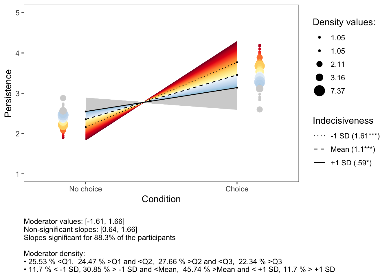

How to interpret this output?

The output of this two-way interaction figure provides several sources of information.

In the figure itself:

the (classic) ‘+- standard deviation’ lines
a blue line representing the slope of the lowest value of the moderator
a red line representing the slope of the highest value of the moderator
a grey area going from the minimum to the maximum value of the moderator
a dark grey area representing all slopes for which the interaction effect is not significant (based on the Johnson-Neyman interval)

On the right, we have numerical information in the legend, showing the minimum and maximum value of the moderator, the numerical value of the Johnson-Neyman interval and the standardized simple slope coefficients (with statistic) for the slopes of the +- 1 standard deviations.

As can be noticed in the figure, it is important to have a full overview of the interaction effect, doing this by including the Johnson-Neyman interval. Based on solely the standard deviation values, we would have thought that “the lower one’s indecisiveness, the more persistence is reported when choice was provided”. However, we see that this effect is not significant for those having (standardized) values on indecisiveness higher than 0.64. From then on, the effect of having choice or not is non-significant on one’s intended persistence.

Multilevel Modeling

Both the summaRy and inteRplot functions are also applicable for multilevel modeling, when using the lmer function of the lme4 package. An example:

library(lme4); library(lmerTest); library(CaviR)

model <- lmer(Depression ~ Dysregulation.c*Integration.c + (1|ID), data=datamultilevel)
summaRy(model)

Predictors	coefficients	β	std. error	t-value	p-value
(Intercept)	1.69	0.00	0.01	293.68	<.001	***
Dysregulation.c	0.55	0.64	0.01	69.99	<.001	***
Integration.c	-0.10	-0.10	0.01	-10.92	<.001	***
Dysregulation.c:Integration.c	-0.06	-0.05	0.01	-5.72	<.001	***

Random effects:
group	Std. Dev.
ID	0.37
Residual	0.30

ANOVA:
	Sumsq	Meansq	(NumDF, DenDF)	F stat	partial η2	VIF
Dysregulation.c	459.54	459.54	(1.00, 7350.68)	4898.52, p = <.001	0.40	1.04
Integration.c	11.18	11.18	(1.00, 7350.99)	119.17, p = <.001	0.02	1.15
Dysregulation.c:Integration.c	3.07	3.07	(1.00, 7271.74)	32.71, p = <.001	0.00	1.11
Residuals	292.721	0.04	7355

Info: 7355 observations, (0) missing obs. deleted
AIC = 9984.01, BIC = 10025.43
R2 conditional = 0.76, R2 marginal = 0.4
ICC = 0.59

library(CaviR)
inteRplot(model,
          pred = 'Dysregulation.c',
          mod = 'Integration.c',
          outcome = 'Depression',
          xaxis = 'Dysregulation',
          moderator = 'Integration',
          miny = 1,
          maxy = 4,
          xlabels=c('Low','High'))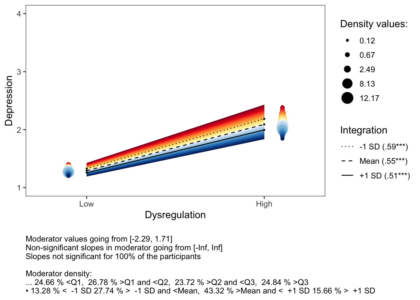

In this interaction effect, there are no non-significant (dark grey) slopes because the interaction effect is significant for each of the moderator’s values.

References

Cohen, Jacob. 2013. Statistical Power Analysis for the Behavioral Sciences. Academic Press.